Abstract Strategy Tree

Table of Contents

• Overview
• AST Node
• Asset Node
• Logical Node
• Example
• Exchange View Node
• Allocation Node

Overview

This is an overview of how to build and structure algorthmic trading strategies in Atlas. As a reminder, Atlas is a is a high performance Algorthmic Trading Backtesting library written in C++23 desigened to be horizontally scalable to operate over large asset universes with mutliple strategies simultaneously. For more info see the Install and ‘What is Atlas’ tabs.

The core of Atlas is an idea taken from compilers and shares its acronym, the Abstract Strategy Tree (AST). In compilers, an Abstract Syntax Tree is a hierarchical representation of the syntactic structure of code in programming languages. Each node in the tree represents a construct in the source code, such as expressions, statements, or declarations. ASTs are commonly used in compilers, interpreters, and static code analysis tools to analyze, transform, or generate code.

Here we use the AST to define a quantitative strategy as tree made up of small reusable, and shareable nodes. This post will give a complete overview of the AST, how it works on the C++ side, what it is designed for, and how it can be extended. To do this we will implement the Super Trend indicator strategy described by the creator of Vector BT here. The basic idea is this taken from their page:

“SuperTrend is a trend-following indicator that uses Average True Range ATR and median price to define a set of upper and lower bands. The idea is rather simple: when the close price crosses above the upper band, the asset is considered to be entering an uptrend, hence a buy signal. When the close price crosses below the lower band, the asset is considered to have exited the uptrend, hence a sell signal.”

You can check out the full formula for the Super Trend indicator, but it is quite involved so it is a good example to show how the AST works.

AST Node

Atlas makes heavy use of object oriented programming, and the AST is no exception. Skipping the lowest level, we start with the StrategyBufferOpNode, a stripped down version is seen below. This node defines the interface for any node the operates over a reference to an eigen vector, which could be an array of portfolio weights, a row of data, a boolean mask, or more.

//============================================================================
export class StrategyBufferOpNode
	: public OpperationNode<void, LinAlg::EigenRef<LinAlg::EigenVectorXd>> {

protected:
	Exchange& m_exchange;

	StrategyBufferOpNode(
		NodeType t,
		Exchange& exchange,
		Option<ASTNode*> parent
	) :
		OpperationNode<void, LinAlg::EigenRef<LinAlg::EigenVectorXd>>(t, parent),
		m_exchange(exchange)
	{}

public:
	virtual ~StrategyBufferOpNode() = default;
    virtual evaluate(LinAlg::EigenRef<LinAlg::EigenVectorXd> target) noexcept = 0;
};

Asset Node

The purpose of the AST is to set the target portfolio weights for a strategy according to some logic or function. To do this we opperate over Eigen vector’s, or more importantely references to them. Each node will take in a reference to an Eigen Vector, and update it accordingly. The simplest operations are asset opperations which are designed to operate element wise over all asset’s listed on an exchange to generate signal values. The most basic is the read op, with copies over a row of data from the exchange onto the target vector

//============================================================================
export class AssetReadNode final
	: public StrategyBufferOpNode
{
private:
	size_t m_column;
	int m_row_offset;
	size_t m_warmup;

public:
	AssetReadNode(size_t column, int row_offset, Exchange& exchange) noexcept;
	void evaluate(LinAlg::EigenRef<LinAlg::EigenVectorXd> target) noexcept override
    {
      auto slice = m_exchange.getSlice(m_column, m_row_offset);  
      target = slice;
    }

Data is stored in the exchange as one massive Eigen matrix in column major order. Each row is an asset, the columns are stored in consecutive order. This read op takes in column and a row offset and returns the appropriate column from the Exchange’s data matrix. In the example below, if we are at t(1) and we ask for Close column offset by -1, the target vector will now hold [150.25, 55.75, 800.5]

Asset	Close (t0)	Feature 1 (t0)	Close (t1)	Feature 1 (t1)
AAPL	150.25	0.75	155.50	0.80
CSCO	55.75	0.60	57.20	0.65
TSLA	800.50	0.45	850.75	0.50

We can now build a binary op node by combining two read ops, and arithmatic op type.

//============================================================================

export class AssetOpNode final
	: public StrategyBufferOpNode
{
private:
	SharedPtr<StrategyBufferOpNode> m_asset_op_left;
	SharedPtr<StrategyBufferOpNode> m_asset_op_right;
	LinAlg::EigenVectorXd m_right_buffer;
	AssetOpType m_op_type;
	size_t warmup;

public:
    //============================================================================
	AssetOpNode(
		SharedPtr<StrategyBufferOpNode> asset_op_left,
		SharedPtr<StrategyBufferOpNode> asset_op_right,
		AssetOpType op_type
	) noexcept;

//============================================================================
    void evaluate(LinAlg::EigenRef<LinAlg::EigenVectorXd> target) noexcept override
{
	m_asset_op_left->evaluate(target);
	m_asset_op_right->evaluate(m_right_buffer);

	assert(target.size() == m_right_buffer.size());
	switch (m_op_type)
	{
	case AssetOpType::MULTIPLY:
		target = target.cwiseProduct(m_right_buffer);
		break;
    }
    ...
}

By the design of the Exchange’s data Eigen matrix, these columns are stored next to each other in column major format, making for fast access. An interesting thing to note here, is that the assetp op node has to store an aditional buffer so that that the target can properly evaluated. The left node writes into the target, the right writes into the buffer, then the target is reassigned.

The ST also uses ATR (average true range). You could build that from a series of blocks, but here we cheat and defined and ATR node, additionally the block computes the entire ATR matrix at instantiation

//============================================================================
void
ATRNode::build() noexcept
{
	if (m_window > m_exchange.getTimestamps().size() || m_window == 0)
	{
		return;
	}

	enableCache();
	auto const& data = m_exchange.getData();
	size_t col_count = m_exchange.getHeaders().size();

	size_t tr_idx = 0;
	double alpha = 1 / static_cast<double>(m_window);
	size_t timestamp_count = m_exchange.getTimestamps().size();
	size_t asset_count = m_exchange.getAssetCount();
	Eigen::VectorXd tr0 = Eigen::VectorXd::Zero(asset_count);
	Eigen::VectorXd tr1 = Eigen::VectorXd::Zero(asset_count);
	Eigen::VectorXd tr2 = Eigen::VectorXd::Zero(asset_count);
	for (size_t i = 0; i < timestamp_count; ++i)
	{
		size_t high_idx = i * col_count + m_high;
		size_t low_idx = i * col_count + m_low;
		size_t close_idx = i * col_count + m_close;

		if (i == 0)
		{
			cacheColumn(i) = (data.col(high_idx) - data.col(low_idx)).cwiseAbs();
			continue;
		}

		tr0 = (data.col(high_idx) - data.col(low_idx)).cwiseAbs();
		tr1 = (data.col(high_idx) - data.col(close_idx - col_count)).cwiseAbs();
		tr2 = (data.col(low_idx) - data.col(close_idx - col_count)).cwiseAbs();
		cacheColumn(i) = alpha * tr0.cwiseMax(tr1).cwiseMax(tr2) + (1 - alpha) * cacheColumn(i - 1);
	}
}

Every node as the option of being cached, which at every time stamp writes the output of the ast node target into a column of an eigen matrix stored by the node. Here we take advantage of that and simply build the whole thing and cache it as we go. At simulation time the ATR node will simply call into the Cache which is and Eigen Matrix managed parent by the base class implementation

//============================================================================
LinAlg::EigenRef<LinAlg::EigenVectorXd>
StrategyBufferOpNode::cacheColumn(Option<size_t> col) noexcept
{
	if (col)
	{
		assert(col.value() < static_cast<size_t>(m_cache.cols()));
		return m_cache.col(col.value());
	}
	if (m_cache.cols() > 1)
	{
		size_t col_idx = m_exchange.currentIdx();
		return m_cache.col(col_idx);
	}
	if (m_cache.cols() == 0)
	{
		size_t rows = m_exchange.getAssetCount();
		m_cache.resize(rows, 1);
		m_cache.setZero();
		return m_cache.col(0);
	}
	return m_cache.col(0);
}

//============================================================================
void
ATRNode::evaluate(LinAlg::EigenRef<LinAlg::EigenVectorXd> target) noexcept
{
	target = cacheColumn(m_exchange.currentIdx());
}

This has it’s ups and down. For starters it is fast because you are accessing memory sequentially all at once in a predictable fashion. On the other hand it requires loading the entire ATR matrix into memory at the start, okay for this example, but if you want to test different ATR params this will impact memory usage.

Logical Node

To buld the ST indicator we also need a way to do element wise comparison of two eigen vectors For that we use the AssetIfNode. This is a fairly simply block,

//============================================================================
export class AssetIfNode final
	: public StrategyBufferOpNode
{
private:
	LinAlg::EigenVectorXd m_buffer;
	AssetCompType m_comp_type;
    SharedPtr<StrategyBufferOpNode> m_right_eval;
	SharedPtr<StrategyBufferOpNode> m_left_eval;

    ...

    void evaluate(LinAlg::EigenRef<LinAlg::EigenVectorXd> target) noexcept override
    {
        m_left_eval->evaluate(target);
        m_right_eval->evaluate(m_buffer);

         switch (m_comp_type) {
            case AssetCompType::GREATER_EQUAL:
			    target = (target.array() >= m_buffer.array()).cast<double>();
			break;
            ...
         }
    }

The node again has a buffer, and then a left and right eval. when the if node is evaluated, it executes it’s left and right node, then compares them accordingly. The result, is overwriting the target vector to 1 where the condition is true, 0 else. This does end up eating the left and right signal, introduces redundency in some case, but in ours it is okay, because we want the true and false evaluations to map to a seperate value not the actual values being compared in the if statement. To do that we use the AssetCompNode

constexpr size_t RIGHT_EVAL_IDX = 0;
constexpr size_t TRUE_EVAL_IDX = 1;
constexpr size_t FALSE_EVAL_IDX = 2;

//============================================================================
export class AssetCompNode final
	: public StrategyBufferOpNode
{
private:
	LinAlg::EigenMatrixXd m_buffer;
	LogicalType m_logical_type;
	SharedPtr<StrategyBufferOpNode> m_right_eval;
	SharedPtr<StrategyBufferOpNode> m_left_eval;
	SharedPtr<StrategyBufferOpNode> m_true_eval;
	SharedPtr<StrategyBufferOpNode> m_false_eval;

    ...

    void evaluate(
	LinAlg::EigenRef<LinAlg::EigenVectorXd> target
) noexcept
{
	m_left_eval->evaluate(target);
	m_right_eval->evaluate(m_buffer.col(RIGHT_EVAL_IDX));
	m_true_eval->evaluate(m_buffer.col(TRUE_EVAL_IDX));
	m_false_eval->evaluate(m_buffer.col(FALSE_EVAL_IDX));
	switch (m_logical_type) {
		case LogicalType::AND:
			target = ((target.array() != 0) && (m_buffer.col(RIGHT_EVAL_IDX).array() !=0))
				.select(m_buffer.col(TRUE_EVAL_IDX), m_buffer.col(FALSE_EVAL_IDX));
		case LogicalType::OR:
			target = ((target.array() != 0) || (m_buffer.col(RIGHT_EVAL_IDX).array() !=0))
				.select(m_buffer.col(TRUE_EVAL_IDX), m_buffer.col(FALSE_EVAL_IDX));
			break;
	}
}

To do this, we need a bigger buffer. We have 4 sup expression representing the left comparions, the right comparions, the true value, and the false value. A full example of the ST indicator in python will follow which shows this in action, but for example look at the ST Final Upper Band:

1. BASIC UPPERBAND = (HIGH + LOW) / 2 + Multiplier * ATR

2. FINAL UPPERBAND = IF (Current BASIC UPPERBAND Less Than Previous FINAL UPPERBAND) or (Previous Close Greater Than Previous FINAL UPPERBAND) THEN Current BASIC UPPERBAND ELSE Previous FINAL UPPERBAND

Example

Skipping over the ATR (average true range), and Median node, and we have what is needed to build the ST indicator. For simplicity sake we write in python taking advtange of the AtlasPy bindings. Let’s start by making the lower and upper bands defined as

1. BASIC UPPERBAND = (HIGH + LOW) / 2 + Multiplier * ATR
2. BASIC UPPERBAND = (HIGH + LOW) / 2 - Multiplier * ATR

This is confusing so now we look at an example

atr_node = ATRNode.make(
    exchange,
    "High",
    "Low",
    14
) 
median_node = AssetMedianNode.make(
    exchange,
    "High",
    "Low",
)
lower_band = AssetOpNode.make(
    median_node,
    AssetScalerNode(atr_node, AssetOpType.MULTIPLY, multiplier),
    AssetOpType.SUBTRACT
)
upper_band = AssetOpNode.make(
    median_node,
    AssetScalerNode(atr_node, AssetOpType.MULTIPLY, multiplier),
    AssetOpType.ADD
)

This intial band is pretty straightforward, note that we didn’t look at the scaler node but it simply does a scaler arithmatic op component wise on it’s input, in this case the ATR. One note above, the ATR is by default built eagerly on creation and is stored in the exchange instance. So in this case each band holds a shared pointer to the same node and takes from the cached data at simulation time.

Looking now at the final band, we use the final upper band definition defined above.

# ===== Upper Band =====
upper_band = AssetOpNode.make(
    median_node,
    AssetScalerNode(atr_node, AssetOpType.MULTIPLY, multiplier),
    AssetOpType.ADD
)
upper_left_cond = AssetIfNode(
    upper_band,
    AssetCompType.LESS,
    DummyNode(exchange)
)
upper_right_cond = AssetIfNode(
    previous_close,
    AssetCompType.GREATER, 
    DummyNode(exchange)
)
final_upper_band = AssetCompNode(
    upper_left_cond,
    LogicalType.OR,
    upper_right_cond,
    upper_band,
    DummyNode(exchange)
)
lagged_final_upper_band = final_upper_band.lag(1)
upper_left_cond.swapRightEval(lagged_final_upper_band)
upper_right_cond.swapRightEval(lagged_final_upper_band)
final_upper_band.swapFalseEval(lagged_final_upper_band)

ST is unique in that it is a recursive algorithm that relies on the previous value. So for that, we build using a dummy, and then use the lag function to create a lagged op on the final band, then swap that back in to the final upper band. Note these are all shared pointers due to pybind11, so when you swap upper_left_cond you are swapping it into the instance held by the final upper band.

Exchange View Node

Now to implement the strategy. This is more complex then simple uniform allocation, it goes long when the close crosses above the final upper band and it goes short when it crosses below. This is more difficult than a moving average cross over as the entry and exit are only true at a single moment in time rather than over a period, (i.e. while close is above 50ma). To do this we use the signal feature of Atlas combined with filters.

spread_upper = AssetOpNode.make(close, final_upper_band, AssetOpType.SUBTRACT)
spread_lower = AssetOpNode.make(close, final_lower_band, AssetOpType.SUBTRACT)
spread_filter_up = ExchangeViewFilter(ExchangeViewFilterType.GREATER_THAN, 0.0)
spread_filter_down = ExchangeViewFilter(ExchangeViewFilterType.LESS_THAN, 0.0)

We start by building two spread nodes comparing the close to the final lower and upper bands, then we create two filters. Filters are fairly straightforward, simply flipping values in the vector to NaN if the condition is false. The more complex part, is building and chaining two exchange views

The exchange view is another StrategyBufferNode and is the last in the chain of evaluation before the portfolio allocations are generated. It holds a single StrategyBufferOpNode to evaluate the generates the signals.

//============================================================================
export class ExchangeViewNode
	final
	: public StrategyBufferOpNode
{
private:
	Option<SharedPtr<ExchangeViewNode>> m_left_view = std::nullopt;
	SharedPtr<StrategyBufferOpNode> m_asset_op_node;
	Vector<SharedPtr<ExchangeViewFilter>> m_filters;
	LinAlg::EigenVectorXd m_buffer;
public:
	ATLAS_API ~ExchangeViewNode() noexcept;

	//============================================================================
	ATLAS_API ExchangeViewNode(
		SharedPtr<Exchange> exchange,
		SharedPtr<StrategyBufferOpNode> asset_op_node,
		Option<SharedPtr<ExchangeViewNode>> left_view
	) noexcept;

Normally, with a single exchange view it’s only roll is to exexcute the AST, generate signals, and apply any filters. But when we pass in a left view it will operate as a signal. Under this scenario we assume that the left and right view can not both be non-Nan at the same time. We default to take right view if it is non-Nan and then we hold the position untill the left view flips to non-Nan and we switch.

//============================================================================
void
ExchangeViewNode::evaluate(LinAlg::EigenRef<LinAlg::EigenVectorXd> target) noexcept
{
    // on evaluation start ExchangeViewd is passed in the current weights vector to write over. We start by evaluating the child AST operation on the target and applying any filters.
    m_asset_op_node->evaluate(target);
    if (m_filters.size()) {
        filter(target);
    }

    // If operating ev as a signal, then we assume that the left and right view cannot be non-Nan
    // at the same time. We only update the EV when the opposing view is non-Nan.
    if (m_as_signal && m_left_view)
    {
        // copy over the previous ev signals to a temp buffer
        LinAlg::EigenVectorXd temp = m_buffer;

        // evaluate the left view over the ev buffer
        (*m_left_view)->evaluate(m_buffer);

        // loop over assets and compare the left and right signal
        for (int i = 0; i < m_buffer.size(); i++)
		{
            // if left signal not nan default take that
            if (!std::isnan(m_buffer(i)))
            {
                if (m_buffer(i) * temp(i) > 0)
                {
                    target(i) = temp(i);
                }
                else
                {
                    target(i) = m_buffer(i);
                }
            }
            // else if previous signal not nan take that. NOTE: assume that if the main ev signal
            // evaluates to NaN we still are in the position untill the right signal fires.
            else if (!std::isnan(temp(i)))
			{
                if (target(i) * temp(i) > 0 || std::isnan(target(i)))
                {
                    target(i) = temp(i);
                }
			}
		}
        // copy over the final output signal into the ExchangeView's buffer
        m_buffer = target;
    }
}

Now we can build our signal using two exchange views

exchange_view_down = ExchangeViewNode.make(exchange, spread_lower, spread_filter_down)
exchange_view_up = ExchangeViewNode.make(exchange, spread_upper, spread_filter_up, exchange_view_down)

Now exchange_view_up holds the final signal output from our supertrend strategy. It will hold (close - final upper band) if that value is greater than 0, else it will hold (close - final lower band) if that value is less than 0. Note it will continue to hold the previous value untill the opposing signal fires, like [10.23,10.23,10.23,-1.3,-1.3] etc. Showing We were long from t0 to t2, then flipped to short.

Allocation Node

To generate the final allocations, we look at the AllocationNode. The allocation node holds and exchange view and is a pure virtual class that is takes in the signal generated by the exchange view, and transforms them into portfolio allocations as well as manage things like, stop loss / take profit, volatilty scaling and targeting, and more.

Skipping over a lot of the base class functionality of it, the core is the virtual evaluteChild method which in this case dynamically allocates the weights based on the exchange view output.

//============================================================================
void
AllocationNode::evaluateChild(LinAlg::EigenRef<LinAlg::EigenVectorXd> target) noexcept
{
	// evaluate the exchange view to calculate the signal
	m_exchange_view->evaluate(target);

	// calculate the number of non-NaN elements in the signal
	size_t nonNanCount = target.unaryExpr([](double x) { return !std::isnan(x) ? 1 : 0; }).sum();
	double c;
	if (nonNanCount > 0) {
		c = (1.0) / static_cast<double>(nonNanCount);
	}
	else {
		c = 0.0;
	}

	switch (m_impl->m_type) {
		case AllocationType::NLARGEST:
		case AllocationType::NSMALLEST:
		case AllocationType::UNIFORM: {
			target = target.unaryExpr([c](double x) { return x == x ? c : 0.0; });
			break;
		}
		case AllocationType::CONDITIONAL_SPLIT: {
			// conditional split takes the target array and sets all elemetns that 
			// are less than the alloc param to -c and all elements greater than the
			// alloc param to c. All other elements are set to 0.0
			target = (target.array() < *m_impl->m_alloc_param)
				.select(-c, (target.array() > *m_impl->m_alloc_param)
					.select(c, target));
			target = target.unaryExpr([](double x) { return x == x ? x : 0.0; });
			break;
		}
		case AllocationType::NEXTREME: {
			assert(false);
		}
	}
}

This is the core function of the allocation node but it also can scale weights accordingy to volatility, target levels of portfolio volatility, apply commissions and more, all of which is defined through the AST. One example of this the TradeLimitNode which defines stop loss and take profit limits and is quite interesting

//============================================================================
export class TradeLimitNode final 
	: public OpperationNode<void,  LinAlg::EigenRef<LinAlg::EigenVectorXd> , LinAlg::EigenRef<LinAlg::EigenVectorXd>,  LinAlg::EigenRef<LinAlg::EigenVectorXd>>
{
	friend class AllocationBaseNode;

private:
	Exchange const& m_exchange;
	TradeLimitType m_trade_type;
	UniquePtr<TradeLimitNodeImpl> m_impl;
	bool m_is_first_step = true;

	void reset() noexcept;

public:
	ATLAS_API TradeLimitNode(
		AllocationBaseNode* parent,
		TradeLimitType trade_type,
		double limit
	) noexcept;

	void evaluate(
		 LinAlg::EigenRef<LinAlg::EigenVectorXd> pnl,
		 LinAlg::EigenRef<LinAlg::EigenVectorXd> current_weights,
		 LinAlg::EigenRef<LinAlg::EigenVectorXd> previous_weights
	)noexcept override;

Node this does not inherit from StrategyBufferOp like the rest, and is intead an Operation Node that takes in the current pnl of a strategy, the current taget weights, and the previous weights and flips the current weights that exceede the thresholds back to 0.

//============================================================================
void TradeLimitNode::evaluate(
	 LinAlg::EigenRef<LinAlg::EigenVectorXd> pnl,
	 LinAlg::EigenRef<LinAlg::EigenVectorXd> current_weights,
	 LinAlg::EigenRef<LinAlg::EigenVectorXd> previous_weights
) noexcept
{
	// in the first step we can't have pnl as allocation node is evaluated after the 
	// portfolio is priced. And it would cause index error trying to get the previous steps
	// returns as we see below.

	if (m_is_first_step)
	{
		m_is_first_step = false;
	}
	else
	{
		// Trade limit node evaluate is called before the allocation node updates.
		// Therefore, current_weights hold the weights that were used for the most 
		// recent evaluation. So we need to update the trade pnl vector to adjust the pnl
		// Stat by pulling in the previous market returns
		auto const& previous_returns = m_exchange.getReturnsScalar();

		// multiply 1 + returns to get the new price using the m_pnl buffer
		pnl = pnl.cwiseProduct(previous_returns);

		// switch on the trade type to zero out weights as required. For stop loss
		// we zero out the weights when the pnl is less than the limit. For take profit
		// we zero out the weights when the pnl is greater than the limit. Add an additional
		// comparison to 0.0 to prevent the new weights from being zeroed out beforehand
		if (isTradeTypeSet(TradeLimitType::STOP_LOSS))
		{
			current_weights = current_weights.array().cwiseProduct(
				((pnl.array() > m_impl->m_stop_loss) || (pnl.array() == 0.0)).cast<double>()
			);
		}
		if (isTradeTypeSet(TradeLimitType::TAKE_PROFIT))
		{
		current_weights = current_weights.array().cwiseProduct(
				((pnl.array() < m_impl->m_take_profit) || (pnl.array() == 0.0)).cast<double>()
			);
		}
	}

	// init the pnl trade vector to 1 where the trade pct switched sign or 
	// went from 0 to non-zero
	pnl = (
		(current_weights.array() * previous_weights.array() < 0.0f)
		||
		(previous_weights.array() == 0) && (current_weights.array() != 0)
		)
		.select(1.0f, pnl);

	// update closed trade. If the current weight is 0 and the previous weight is not 0
	// then zero out the pnl vector
	pnl = (
		(current_weights.array() == 0)
		&& 
		(previous_weights.array() != 0)
		)
		.select(0.0f, pnl);
}

We don’t make use of that here, but adding this functionality is simple given an existing AST. Finally, putting it altogether into a strategy and running it:

allocation_signal = AllocationNode.make(
    exchange_view_up,
    AllocationType.CONDITIONAL_SPLIT,
    0.0,
    -1
)
strategy_node_signal = StrategyNode.make(allocation_signal, portfolio)
strategy = hydra.addStrategy(Strategy(strategy_id, strategy_node_signal, 1.0), True)
strategy.enableTracerHistory(TracerType.NLV)
strategy.enableTracerHistory(TracerType.ORDERS_EAGER)
hydra.run()

To look at the actual signal we can inspect the AST nodes cache.

path = os.path.join(exchange_path,"BTC-USD.csv")  
df = pd.read_csv(path)
df["final_upper_band"] = final_upper_band.cache()[0]
df["final_lower_band"] = final_lower_band.cache()[0]
df["ev"] =  exchange_view_up.cache()[0]
df["spread_lower"] = df["Close"] - df["final_lower_band"]

df["Date"] = pd.to_datetime(df["Date"])
df.set_index("Date", inplace=True)
df.index = df.index.tz_localize(None)

asset_id = 0
orders = strategy.getTracer().getOrders()
orders = [o.to_dict() for o in orders]
df_orders = pd.DataFrame(orders)
df_orders["fill_time"] = pd.to_datetime(df_orders["fill_time"])
df_orders = df_orders[df_orders["asset_id"] == asset_id]
df_orders.set_index("fill_time", inplace=True)

Above we load in the band’s cache as well as the strategy’s orders. Some of the code needed to enable this was left out in the cells above. To see the full notebook implementation, see the repo

To make sure we are doing it right we can look at the signal and the orders that were placed

n = 200
df_sub = df.iloc[:n]
df_sub_max_time = df_sub.index.max()
df_orders_sub = df_orders[df_orders.index <= df_sub_max_time]

buys = df_orders_sub[df_orders_sub["quantity"] > 0]
sells = df_orders_sub[df_orders_sub["quantity"] < 0]

plt.figure(figsize=(12,6))
plt.plot(df_sub["Close"], label="Close")
plt.plot(df_sub["final_upper_band"], label="Final Upper Band")
plt.plot(df_sub["final_lower_band"], label="Final Lower Band")
plt.scatter(buys.index, buys["fill_price"], label="Buy", marker="^", color="g")
plt.scatter(sells.index, sells["fill_price"], label="Sell", marker="v", color="r")
plt.title("Upper Band")
plt.legend()
plt.show()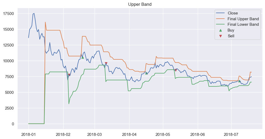

If you time the function execution you’ll see that this situation underpeforms in speed when operating over a single asset, but has great scaling horizontally. This is not particulary suprising, this AST implementation is designed to be flexiable, compared to something like VectorBT’s numba jit method. I found bumping up the asset count from 1 to 11 in this toy example to have little effect on the total runtime for the overall simulation (3 ms -> 4.5ms).