Grid Search, Volatility Scaling/Target, and GUI improvement

Engine features and GUI improvement

Intro
Volatility
Grid Search

Intro

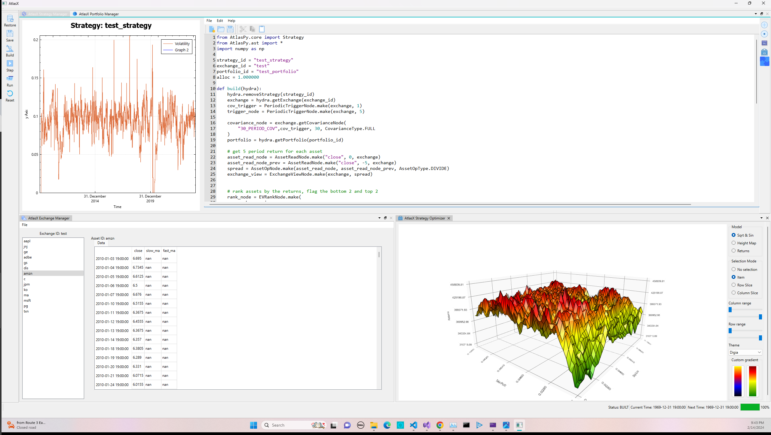
In my previous post I introduced many different features to improve the feature set of the Atlas backtesting engine as well as introduce a GUI to help faciliate the creation of new strategies. In the past two weeks the GUI has come a long way, mainly in the domain of visualization as you can see above. I have switched from QTCharts to QCustomPlot for the 2d visualization, and added QT’s data visualtion library for 3d visualition, more on this below.

In addition to the GUI, I added a couple of key features as well as stabalized and refactor the existing API. We will go into detail below, but at high level that includes improving the Abstract Strategy Tree usability, implementing volatility targeting and scaling, and child strategies and grid search techniques for optimization. We will start off by looking at the new aditions in the area of volatility.

Volatility

Volatility plays a key part in any quantitative trading strategy especially in a framework such at Atlas that revolves around horizontally scaling strategies and target weight allocations, (i.e. strategies desigend to operate over large asset universes compared to one that is designed to trade the SP500 eminis).

To implement any sort of functionality revolving around vol you need a covariance matrix. More importantly one that evovles throughout time as vol is not constant nor are correlations. Thus we define a new AST node type containing a covariance measure

//============================================================================
export class CovarianceNodeBase : public StatementNode
{
private:
	bool m_cached = false;
	size_t m_warmup = 0;
protected:
	size_t m_lookback_window = 0;
	SharedPtr<TriggerNode> m_trigger;
	Exchange& m_exchange;
	LinAlg::EigenMatrixXd m_covariance;
	void enableIncremental() noexcept { m_incremental = true; }

public:
	CovarianceNodeBase(
		Exchange& exchange,
		SharedPtr<TriggerNode> trigger,
		size_t lookback_window
	) noexcept;

	void reset() noexcept;
    virtual void evaluateChild() noexcept = 0;
	void evaluate() noexcept override;
	SharedPtr<TriggerNode> getTrigger() const noexcept { return m_trigger; }
	Exchange& getExchange() const noexcept { return m_exchange; }
	LinAlg::EigenMatrixXd const& getCovariance() const noexcept { return m_covariance; }

};

As usual I slim down the above code to look at the relevant pieces. Mainly beeing it takes in an exchange to operate over and a trigger that defines the refresh schedule. Calculating the covariance is a relatively expesensive operation so allowing you to do it every N steps instead of every step can save time without sacrificing to much accuracy (at least during low vol periods). Note also this is technically an abstract base class that allows for a child class to define how the covariance matrix is set, for now I only have a standard implemention seen below. An incremental updater is in the works pending numerical stability test.


void
CovarianceNode::evaluateChild() noexcept
{
	size_t start_idx = (m_exchange.currentIdx() - m_lookback_window) + 1;
	auto const& returns_block = m_exchange.getMarketReturnsBlock(
		start_idx,
		m_exchange.currentIdx()
	);
	Eigen::MatrixXd returns_block_transpose = returns_block.transpose();
	m_centered_returns = returns_block_transpose.rowwise() - returns_block_transpose.colwise().mean();
	m_covariance = (m_centered_returns.adjoint() * m_centered_returns) / 
    double(returns_block_transpose.rows() - 1);
}

https://github.com/ntorm1/Atlas/blob/main/modules/ast/RiskNode.cpp

As we are operating over return space in the Atlas engine, the covariance calculation is actually quite straight forward. In essence we take the current idx in the exchange returns block, and then offset it by the covariance lookback to get the returns block containing the N period historical returns for each asset. This block is in column major form, so we have to transpose before applying some linear algebra operations helpfully provided by Eigen. Now any strategy node can use this covariance matrix during it’s execution without repeated calculation, with the parent exchange updating and cacheing it as needed.

To make use of this, we first define an additional AST node type called AllocationWeightNode that takes in a covariance matrix and operates over the strategy buffer to scale the weights by some given measure

//============================================================================
export class AllocationWeightNode : public StrategyBufferOpNode
{
protected:
	SharedPtr<CovarianceNodeBase> m_covariance = nullptr;
	Option<double> m_vol_target = std::nullopt;

protected:
	void targetVol( LinAlg::EigenRef<LinAlg::EigenVectorXd> target) const noexcept;

public:
	virtual ~AllocationWeightNode() noexcept;

	AllocationWeightNode(
		SharedPtr<CovarianceNodeBase> covariance,
		Option<double> vol_target
	) noexcept;
	
	virtual void evaluate( LinAlg::EigenRef<LinAlg::EigenVectorXd> target) noexcept = 0;
	bool getIsCached() const noexcept { return m_covariance->getIsCached(); }
};

This could be any method, for example equal risk contribution is something I would like to add. Either way, this is an important feature as it takes into account the volatility of the indivual assets when determining portfolio allocation. I.e. if we determine the portfolio should go long the top 10 stock by N period returns, we want to scale the weights such that the risk budget for each stock is the same. For now we rely on a simple inverse volaility weighting which scales each weight in the portfolio by the inverse of the volaility, i.e. the covariance matrix diagnol.

//============================================================================
void
InvVolWeight::evaluate( LinAlg::EigenRef<LinAlg::EigenVectorXd> target) noexcept
{
	auto const& covariance = m_covariance->getCovariance();
	auto vol = covariance.diagonal().array().sqrt();
	target = (target.array() / vol.array()).matrix();
	double abs_weight_sum = target.array().abs().sum();
	target = (target.array() / abs_weight_sum).matrix();
	if (m_vol_target)
	{
		targetVol(target);
	}
}

The algorithm itself is not to complicated, simply take the weights scale by the covariance diagonal and renormalize. This does by defintion set the portfolio allocation equal to 1, which might not be desirable. To get around this we add vol targeting. This takes in a double like “0.10” which defines the portfolios target annualized volatility level to be 10%. Note for now this only operates over daily equity space as we assume 252 trading period in a year. Future work would make this more robust.

//============================================================================
void
AllocationWeightNode::targetVol( LinAlg::EigenRef<LinAlg::EigenVectorXd> target) const noexcept
{
	auto const& covariance = m_covariance->getCovariance();
	auto v = (target.transpose() * covariance * target);
	double annualized_vol = std::sqrt(v(0)) * std::sqrt(252);
	double vol_scale = m_vol_target.value() / annualized_vol;
	target *= vol_scale;
}

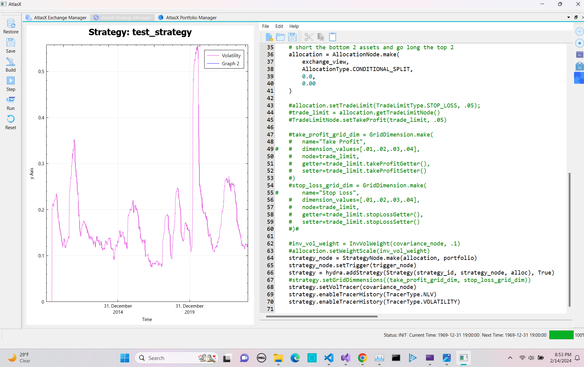
Before we apply the target vol we can look at how the naieve weight allocation’s forward vol looks. In this case we are essentially targeting the strategy to have a net leverage ratio of 1 regardless of volatility, leading to large swings in the forward vol if we don’t apply a vol target.

Now we look at applying weight and vol scaling. All of the above functionality is available via the python wrapper so we can continue to make strategies dynamically. In essence all we have to do it define a covariance node over the strategie’s exchange, and the build a inverse vol weight node

def build(hydra):
	hydra.removeStrategy(strategy_id)
	exchange = hydra.getExchange(exchange_id)
	cov_trigger = PeriodicTriggerNode.make(exchange, 5)
	trigger_node = PeriodicTriggerNode.make(exchange, 10)
	
	covariance_node = exchange.getCovarianceNode(
		"100_PERIOD_COV",cov_trigger, 100, CovarianceType.FULL
	)

    ...
    allocation = AllocationNode.make(
		exchange_view,
		AllocationType.CONDITIONAL_SPLIT,
		0.0,
		0.01
	)

    inv_vol_weight = InvVolWeight(covariance_node, .1)
    allocation.setWeightScale(inv_vol_weight)
    strategy_node = StrategyNode.make(allocation, portfolio)
    strategy = hydra.addStrategy(Strategy(strategy_id, strategy_node, alloc), True)

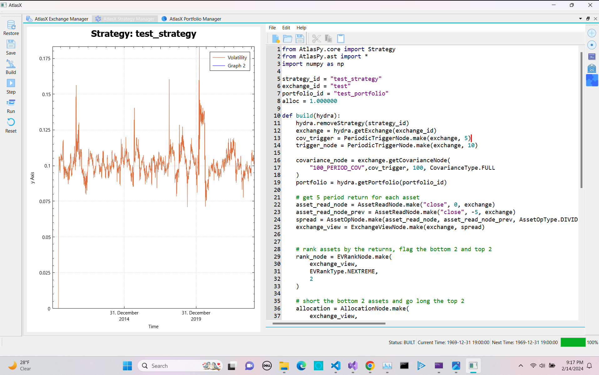
Skipping the actual strategy logic, the above sets a covariance matrix that updates every week and a strategy that updates every two weeks. Note that the trigger nodes and covariance nodes static make function first searches for a corresponding exsisting node on registered to the exchange and returns that if it finds it. Else it creates it. Additionally, we set allocation epsilon to 1% to allow weights to deviate. So while we expect the target vol to be 10%, the number will vary:

If we want to get the actual forward vol closer, we need to update the strategy weights and covariance matrix faster, as well as tighten the weights epsilon. Svelte

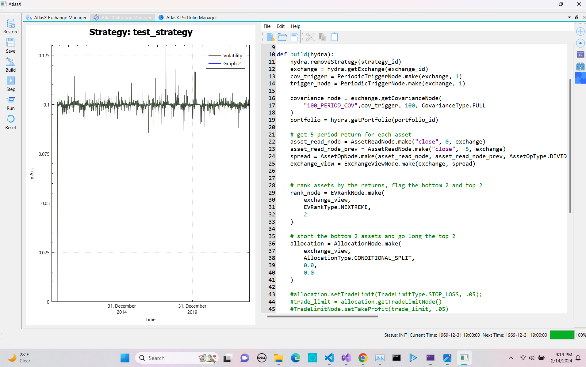
You’ll notice we still don’t see a horizontal line at 10%. The reason for this is that at time t1 the strategy sets the weights with covariance matrix at time t1, but then on the next step forward the strategy is evaluated with the covariance matrix at time t2 which as changed before the strategy updates the weights. Thus we no longer have our target vol. So if the covariance matrix shifts significantly you’ll see deviations.

Grid Search

One of the features I am most excited about is the grid search implementation for strategy hyper parameter evaluation. For now the grid search simply evaluate possible variation of a given abstract strategy tree but does not select or rank them in order to make adjustements to the base strategy. That would be next on my to do.

The implementation of the grid search relies on two new classes, the StrategyGrid and the GridDimension. The latter of which defines a hyperparamter to fit over and a series of values to search over. The basic idea is to supply an AST node, a getter and setter function to tweak the values for, and a range to do it over.

export struct GridDimension
{
    using GetterFuncType = double(*)(SharedPtr<TradeLimitNode>) noexcept;
	using SetterFuncType = void(*)(SharedPtr<TradeLimitNode>, double) noexcept;
    
	String dimension_name;
	size_t dimension_size;
	Vector<double> dimension_values;
	SharedPtr<TradeLimitNode> buffer_node;
	double(*buffer_node_getter)(SharedPtr<TradeLimitNode>);
	void(*buffer_node_setter)(SharedPtr<TradeLimitNode>, double);
	uintptr_t getter_addr;
	uintptr_t setter_addr;
	size_t current_index = 0;

    GridDimension(
	const String& name,
	const Vector<double>& dimension_values,
	const SharedPtr<TradeLimitNode>& node,
	uintptr_t getter,
	uintptr_t setter
) noexcept :
	...
{
	buffer_node_setter = reinterpret_cast<SetterFuncType>(setter);
	buffer_node_getter = reinterpret_cast<GetterFuncType>(getter);
}

This implementation currently operates over a TradeLimitNode as an initial test of the black magic that is the reinterpret_cast. The uintptr_t types are a bit odd, and actually allow you to pass function pointers (dangerously) from python to c++ via pybind11 with no overhead that can adjust the given node at runtime. If you pass a normal function pointer using pybind11, the GIL has to be aquired every time you exectue the function. In this case that will be frequent as the setter will be called N squared times per timestamp.

Instead when constructing the dimension you call a function on the node that returns the address of a static function that can operate on the trade limit nodes. You pass this pointer address to c++ and than create that function pointer on the c++ side. Note if you print it out from python you will see a regular interger. Theortically you can pass in any integer and it won’t raise an exception, but if you don’t pass in these specefic static addresses the program will implode at run time. Something to look into.

Here is what that looks like on the python side.

	allocation.setTradeLimit(TradeLimitType.TAKE_PROFIT, .05)
	trade_limit = allocation.getTradeLimitNode()
	take_profit_grid_dim = GridDimension.make(
		name="Take Profit",
		dimension_values=list(np.linspace(0.01, .05, 50)),
		node=trade_limit,
		getter=trade_limit.takeProfitGetter(),
		setter=trade_limit.takeProfitSetter()
	)
	stop_loss_grid_dim = GridDimension.make(
		name="Stop Loss",
		dimension_values=list(np.linspace(0.01, .05, 50)),
		node=trade_limit,
		getter=trade_limit.stopLossGetter(),
		setter=trade_limit.stopLossSetter()
	)

    ...

    strategy.setGridDimmensions((take_profit_grid_dim, stop_loss_grid_dim))

This defines a hyper parameter space to test over. Namely test every combination of take profit and stop loss from 1% to 5% with 50 steps in between. This operation scales N squared, above we are evualting 2500 different strategies.

So what does this actually do on the C++ side at runtime and how do we evaluate each possiblity while not affecting the base strategy implementation. This is where the StrategyGrid comes in.

//============================================================================
export class StrategyGrid
{
	friend class Strategy;
private:
	Strategy* m_strategy;
	Exchange const& m_exchange;
	std::pair<SharedPtr<GridDimension>, SharedPtr<GridDimension>> m_dimensions;
	LinAlg::EigenMatrix<SharedPtr<Tracer>> m_tracers;
	double* m_weights_grid = nullptr;
	size_t m_asset_count = 0;

	LinAlg::EigenMap<LinAlg::EigenVectorXd> getBuffer(size_t row, size_t col) noexcept;
	size_t gridStart(size_t row, size_t col) const noexcept;
	void reset() noexcept;
	void evaluateGrid() noexcept;
	void evaluateChild(size_t row, size_t col) noexcept;

public:
	StrategyGrid(
		Strategy* strategy,
		Exchange const& exchange,
		std::pair<SharedPtr<GridDimension>, SharedPtr<GridDimension>> m_dimensions
	) noexcept;

The strategy grid takes in a strategy and pair of grid dimensions to operate over and sets up a series of objects to maintain the state of the indivual sub-strategies. First it sets up a matrix of Tracer objects each of each can keep track of PnL, Vol and other attributes for a given sub-strategy. The next is the weights grid, which is a giant buffer of doubles that contains all of the weights for all of the sub-strategies in one continuous piece of memory.

//============================================================================
StrategyGrid::StrategyGrid(
	Strategy* strategy,
	Exchange const& exchange,
	std::pair<SharedPtr<GridDimension>, SharedPtr<GridDimension>> dimensions
) noexcept
:
	...
{
	double initial_cash = strategy->getTracer().getInitialCash();
	size_t row_count = m_dimensions.first->size();
	size_t col_count = m_dimensions.second->size();
	size_t depth = m_asset_count;
	m_tracers.resize(row_count, col_count);
	for (size_t i = 0; i < row_count; ++i)
	{
		for (size_t j = 0; j < col_count; ++j)
		{
			m_tracers(i, j) = std::make_shared<Tracer>(
				*m_strategy,
				exchange,
				initial_cash
			);
		}
	}
	m_weights_grid = new double[row_count * col_count * depth];
	memset(m_weights_grid, 0, row_count * col_count * depth * sizeof(double));
}

In essence each sub strategy requires a double* buffer of size equal to the #assets to maintain the target weight allocation. All of these are stored in continous memory for nice cache coherency. Continuing on to what happens at simulation time, the grid loops over all combinations of parameters, sets the corresponding values onto the trade limit node, evaluates the AST, then replaces the orginal values to continue on. Here we swap

//============================================================================
void
StrategyGrid::evaluateGrid() noexcept
{
	// copy shared pointers to tracers to swap back in after evaluation of grid
	auto tracer = m_strategy->getTracerPtr();

	// loop over grid and use node getters and setters to evaluate the strategy
	// over the parameter space
	size_t row_count = m_dimensions.first->size();
	size_t col_count = m_dimensions.second->size();

	// store the original value of the dimensions
	double original_row_value = m_dimensions.first->getNodeValue();
	double original_col_value = m_dimensions.second->getNodeValue();

	// evaluate the grid strategy with the current market prices and weights
	evaluate();
	for (size_t i = 0; i < row_count; ++i)
	{
		double row_value = m_dimensions.first->getNodeValue();
		m_dimensions.first->set(i);
		for (size_t j = 0; j < col_count; ++j)
		{
			double col_value = m_dimensions.second->dimension_values[j];
			m_dimensions.second->setNodeValue(col_value);
			evaluateChild(i, j);
		}
		m_dimensions.first->setNodeValue(row_value);
	}
	// restore original value of the dimensions for the base strategy
	m_dimensions.first->setNodeValue(original_row_value);
	m_dimensions.second->setNodeValue(original_col_value);
	m_strategy->setTracer(tracer);
}

Here we are swapping in and out the various tracer instances for the indivual strategy grid elements. This tracer contains all the information about strategy evaluation over time and needs to be swapped in an out as we loop over the grid corresponding to the right tracer. So to evaluate the AST using the grid values we evaluate the strategy in place using the grid’s weight buffer.

//============================================================================
void
StrategyGrid::evaluateChild(size_t row, size_t col) noexcept
{
	// AST has been swapped in place, now evaluate strategy using grid's buffers
	auto weights_buffer = getBuffer(
		row,
		col
	);
	// evaluate the strategy with the current market prices and weights using 
	// the grid buffers
	auto tracer = m_tracers(row, col);
	m_strategy->setTracer(tracer);
	m_strategy->step(weights_buffer);
}

One thing to note is that this is attempting to make this run in parralell on multiple threads will give you invalid answers. The grid must be evaluated one at a time as the grid shares the entire AST and just has their own target weight buffer and tracer instance. So if you try and eval two sub strategies at the same time setting different stop loss levels you’ll not get the correct result. On the other hand, we can evaluate them all at the same time by taking advtange of the Eigen map over a matrix

//============================================================================
void
StrategyGrid::evaluate() noexcept
{
	LinAlg::EigenConstColView market_returns = m_exchange.getMarketReturns();
	LinAlg::EigenMap<LinAlg::EigenMatrixXd> weights_grid(
		m_weights_grid,
		m_asset_count,
		m_dimensions.first->size() * m_dimensions.second->size()
	);
	LinAlg::EigenVectorXd portfolio_returns = market_returns.transpose() * weights_grid;
	for (size_t i = 0; i < m_dimensions.first->size(); ++i)
	{
		for (size_t j = 0; j < m_dimensions.second->size(); ++j)
		{
			auto tracer = m_tracers(i, j);
			double nlv = tracer->getNLV();
			tracer->setNLV(nlv * (1.0 + portfolio_returns(i * m_dimensions.second->size() + j)));
			tracer->evaluate();
		}
	}
}

Here we make a view into the weights grid holding the actual allocations of each substrategy and take the product of the market returns to get the indivual portfolio returns of each of the sub strategies. Now can put it together with the full python code being:

from AtlasPy.core import Strategy
from AtlasPy.ast import *
import numpy as np

strategy_id = "test_strategy"
exchange_id = "test"
portfolio_id = "test_portfolio"
alloc = 1.000000

def build(hydra):
	hydra.removeStrategy(strategy_id)
	exchange = hydra.getExchange(exchange_id)
	cov_trigger = PeriodicTriggerNode.make(exchange, 1)
	trigger_node = PeriodicTriggerNode.make(exchange, 5)
	
	covariance_node = exchange.getCovarianceNode(
		"30_PERIOD_COV",cov_trigger, 30, CovarianceType.FULL
	)
	portfolio = hydra.getPortfolio(portfolio_id)
	
	# get 5 period return for each asset
	asset_read_node = AssetReadNode.make("close", 0, exchange)
	asset_read_node_prev = AssetReadNode.make("close", -5, exchange)
	spread = AssetOpNode.make(asset_read_node, asset_read_node_prev, AssetOpType.DIVIDE)
	exchange_view = ExchangeViewNode.make(exchange, spread)

	
	# rank assets by the returns, flag the bottom 2 and top 2
	rank_node = EVRankNode.make(
		exchange_view,
		EVRankType.NEXTREME,
		2
	)

	# short the bottom 2 assets and go long the top 2
	allocation = AllocationNode.make(
		exchange_view,
		AllocationType.CONDITIONAL_SPLIT,
		0.0,
		0.025
	)
	
	allocation.setTradeLimit(TradeLimitType.STOP_LOSS, .05)
	trade_limit = allocation.getTradeLimitNode()
	TradeLimitNode.setTakeProfit(trade_limit, .05)
	
	take_profit_grid_dim = GridDimension.make(
		name="Take Profit",
		dimension_values=list(np.linspace(0.01, .1, 50)),
		node=trade_limit,
		getter=trade_limit.takeProfitGetter(),
		setter=trade_limit.takeProfitSetter()
	)
	stop_loss_grid_dim = GridDimension.make(
		name="Stop Loss",
		dimension_values=list(np.linspace(0.01, .1, 50)),
		node=trade_limit,
		getter=trade_limit.stopLossGetter(),
		setter=trade_limit.stopLossSetter()
	)
	
	inv_vol_weight = InvVolWeight(covariance_node, .1)
	allocation.setWeightScale(inv_vol_weight)
	strategy_node = StrategyNode.make(allocation, portfolio)
	strategy_node.setTrigger(trigger_node)
	strategy = hydra.addStrategy(Strategy(strategy_id, strategy_node, alloc), True)
	strategy.setGridDimmensions((take_profit_grid_dim, stop_loss_grid_dim))
	strategy.setVolTracer(covariance_node)
	strategy.enableTracerHistory(TracerType.NLV)
	strategy.enableTracerHistory(TracerType.VOLATILITY)

Running this in that AtlasX editor we see that setting the stop loss and take profit too tight lead to decreased returns, with the sweat spot being around 3-4% stop loss and take profit for this strategy that rebalances on a weekly basis. Also, it takes around 2 seconds to run the entire simulation over the 2500 sub-strategies in the grid in release mode with AVX2 instruction set. Not sure how helpful AVX2 is given these vectors are relatively small but still cool. So that is 3500 time steps for 14 assets and 2500 sub strategies, effectively looping over 122,500,000 candles in 2 seconds, or 60 million candles per second on a single thread.

The next step is to expand this to other nodes to allow for more possibilites, and to select strategies at simulaton time based on their grid ranking at various time steps for true walk forward validation.

Grid Search, Volatility Scaling/Target, and GUI improvement

Engine features and GUI improvement

Table of Contents

Intro

Volatility

Grid Search